From table
15
20
25
30
35
40
45
125
250
500
1k
2k
4k
T
ransmission
Loss
T
L
r
[dB]
Frequency f [Hz]
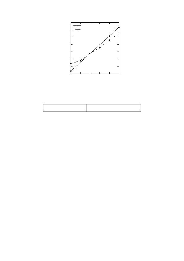
Transmission loss in 1/3 octave band
20 log(ωm)
− 48
10
Figure 6: Transmission loss for random incidence, T L
r
, for a 1 mm thick steel plate, numerically
calculated from T L
r
= 20 log(ωm)
− 48 and compared to data in table
Frequency f
[Hz]
125
250
500
1000
2000
4000
Transmission loss T L
r
[dB]
17
19
24
28
33
38
Table 2: Transmission loss T L
r
for a 1 mm thick steel plate for different frequencies.
The code for figure
set terminal fig monochrome textspecial
set output "plot/transloss2.fig"
# Title and x/y-labels:
set title "Transmission loss in 1/3 octave band"
set xlabel "Frequency $f$ [Hz]" offset 0,character -1
set ylabel "Transmission Loss $TL_r$ [dB]"
# Place legend at top left, change place of text and linetype with "reverse",
# align text left with "Left" and increase spacing between items:
set key top left reverse Left spacing 2
# Used to scale the figure:
set size square 1,1
# Logarithmic x-axis, base 10 (default, though)
set logscale x 10
# xtics sets slightly rotated. Define the tics; ("label" pos, "label" pos, ... )
set xtics rotate by -30 ("125" 125, "250" 250, "500" 500, "1k" 1000, "2k" 2000, "4k" 4000)
plot "data/transloss2.dat" using 1:2 title "$20\\log(\\omega m)-48$" with linespoints 1 5, \
"data/transloss2.dat" using 1:3 title "From table \\ref{tab:transloss2}" with linespoints 2 1
8