From table
25
30
35
40
45
50
55
60
f c
0
1000
2000
3000
4000
5000
6000
20
25
30
35
40
45
50
55
60
f c
0
1000
2000
3000
4000
5000
6000
T
ransmission
Loss
T
L
r
[dB]
Frequency f [Hz]
Transmission loss as a function of frequency
20 log(ωm)
− 48
10 log(1 +
ωm
2ρc
2
)
− 10 log(0.23 · 10 log(1 +
ωm
2ρc
2
))
20
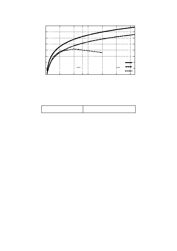
Figure 5: Transmission loss for random incidence, T L
r
, for a 4.5 mm thick steel plate, numerically
calculated from two different equations and compared to table data. Coincidence frequency, f
c
,
is marked in figure and is about 2.6 kHz.
Frequency f
[Hz]
125
250
500
1000
2000
4000
Transmission loss T L
r
[dB]
22
27
34
39
41
38
Table 1: Transmission loss T L
r
for a 4.5 mm thick steel plate for different frequencies.
The code for figure
set terminal fig monochrome textspecial
set output "plot/transloss.fig"
set title "Transmission loss as a function of frequency"
set xlabel "Frequency $f$ [Hz]"
set ylabel "Transmission Loss $TL_r$ [dB]"
# Stops plotting at end of data, not continuing to next xtic or x2tic (x=7000):
set autoscale xfixmax;
set autoscale x2fixmax
# This loads the file containing the coincidence frequency, fc, which is around 2600 Hz.
# The file contains just "fc = 2603" or something like that.
load "data/transloss-fc.dat"
# Add a xtic and x2tic item for the coincidence frequency:
set xtics add ("$fc$" fc);
set x2tics add ("$fc$" fc)
set y2tics
# Set tics on right y-axis.
# Place legend at right bottom and increase spacing between items:
set key right bottom spacing 2.5
set grid
# enable grid, default settings
# Plotting with lines and specified linewidth (lw) = 3:
plot "data/transloss.dat" using 1:2 title "$20\\log(\\omega m)-48$" with lines lw 3, \
"data/transloss.dat" using 1:3 title "$10\\log(1+\\frac{\\omega m}{2\\rho c}^2)-\
10\\log(0.23\\cdot 10\\log(1+\\frac{\\omega m}{2\\rho c}^2))$"\
with lines lw 3, \
"data/transloss-tab.dat" title "From table \\ref{tab:transloss}" with lines lw 3
7